Transition to Turbulence
Created by Ian Nesbitt and Jukes Liu on 2019-02-19. Because this page has some high-resolution animations, it is best viewed on a reliable internet connection.
Welcome to our teaching module on fluid flow past a cylinder!
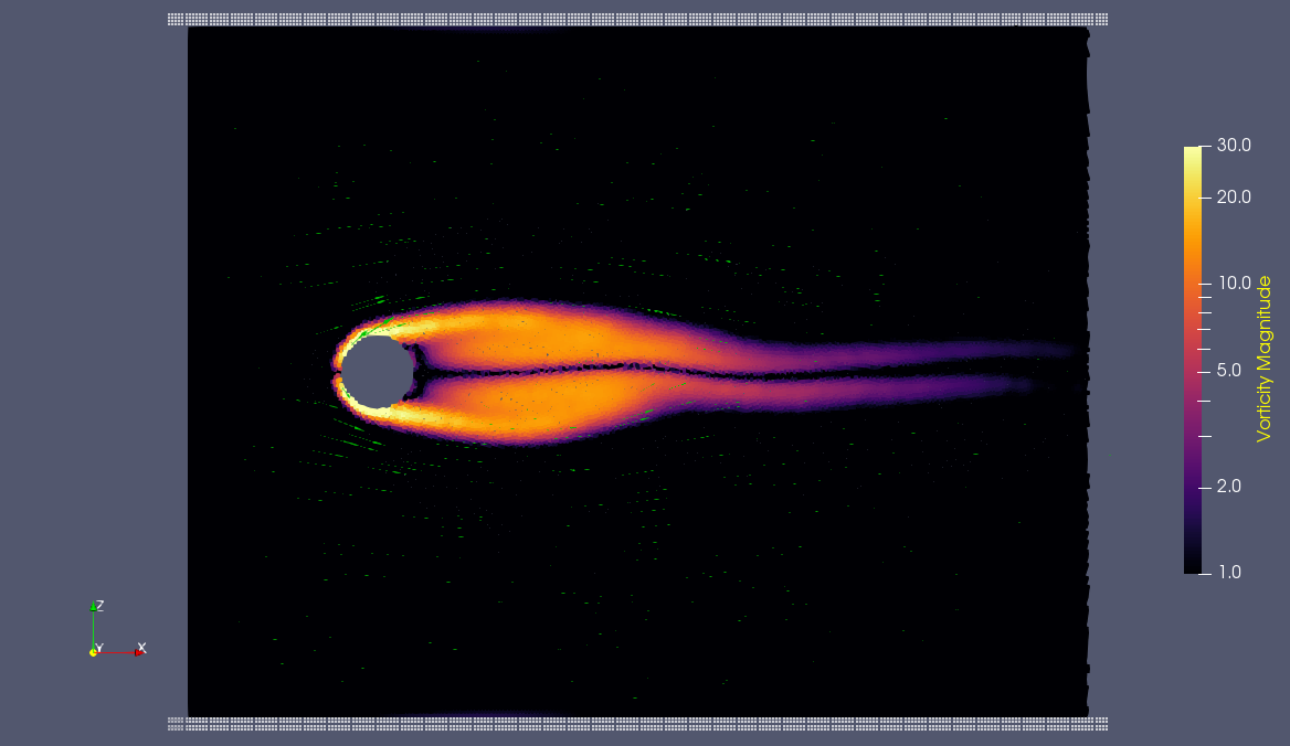
In this module, we will explore the transition to turbulence and learn how viscosity affects the dynamics of a fluid flowing around a cylindrical impediment. We can observe an interesting phenomenon called Von Kármán Vortex Streets at this simulated transition to turbulence. Their naturally-occurring counterparts are fascinating and have many environmental and engineering applications. Below is a snapshot of one of our generated model of water flowing past a cylinder. In this early time-step, we can see an instability begin to develop in the wake of the cylinder.
Contents
Overview
In order to model the transition to turbulence and the effects of changing viscosity on the dynamics of a simple fluid system with a single cylindrical impediment placed in the flow path, we use several modeling tools: COMSOL Multiphysics, Smoothed-Particle Hydrodynamics (SPH), and ParaView. We will describe the model set-up and its physical basis, the differences between the three scenarios with fluids of different viscosities, and several real-world implications. We will move from looking at the behavior of more viscous fluids and move towards fluids with lower viscosities. Note: Viscosity is defined as the measure of a fluid's resistance to deformation.
At the end of the module, you should be able to describe the initial conditions of a system, the transition from laminar to turbulent flow, and the effect viscosity has on the inertia, complexity, and predictability of a system!
First, let's start by learning how to talk about the various components of flow.
Characterizing the fluid dynamics
When we talk about fluid flow, we need to first describe the fluid. Some of the fundamental characteristics of fluid are density, viscosity, compressibility, heat capacity, and thermal conductivity. In this exercise we will ignore the thermal properties entirely, define a constant density and compressibility, and focus most of our attention on how viscosity affects the kinematics of a fluid system.
Compressibility and density are fairly easy to define. Compressibility is the tendency of a fluid to change its volume due to changes in pressure. Since we are not dealing with immense pressure, we assume that compressibility is zero across all models. Density is the quantity of mass per unit volume. For the purposes of this model, we will hold density constant at 1 kg m-3 to try and isolate the effects of viscosity. These parameters will be fed into the Navier-Stokes fluid momentum equation (below) for each location in the model at each time step.
To characterize the motion of particles in the fluid, we must account for the changes in momentum. This Navier-Stokes equation is derived based on the conservation of momentum in a system. It is the foundation of our models. This equation can be broken down into its different terms, which represent the effects of the inertial forces, body forces, viscous forces, and the pressure gradient throughout the system.
This is the basic structure of the Navier-Stokes momentum equation:
Acceleration = Body forces + Shear forces - Pressure gradient
These qualitative terms are represented by some greek symbols which may or may not mean anything to you right now, but we'll break them down for you.
∂v / ∂t = ρg + µ∇2U - ∇P
| where | |
|---|---|
| ∂v | = change in velocity |
| ∂t | = change in time |
| ρ | = density |
| g | = acceleration due to gravity |
| µ | = viscosity |
| ∇2U | = divergence of velocity (gradient) |
| ∇P | = divergence of pressure (gradient) |
The inertial forces (acceleration) is represented by ∂v / ∂t.
On the right hand side of the equation, we have the body forces from density and gravity (ρg), viscous forces from the viscosity property of the fluid (µ∇2U), and the pressure gradient throughout the system (∇P). Each of these forces will influence the acceleration or motion of particles. Can you visualize how these different forces on the right-hand side of the equation might influence a particle's motion?
Solving this equation for each grid point or particle at each time step will define how our fluid will behave in a computational sense. Once our fluid starts to move, we need ways to describe how it is flowing. Fluid flow can be characterized as either laminar or turbulent, which has to do with the predictability of its motion throughout the system. The parameter that is used to describe this characteristic is called the Reynolds number.
Reynolds number
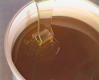
The Reynolds number, Re, is a simple, dimensionless number that represents the flow regime of a fluid. The Reynolds number is a way of representing whether a flow is laminar, transitional, or fully turbulent using numerical values. When flow is laminar, the fluid motion is more uni-directional, smooth, and more predictable. Imagine the flow of molasses being poured out onto a table. Another example would be toothpaste being squeezed out of the tube. Laminar flow is represented by lower Reynolds numbers. When flow is turbulent, fluid motion is more irregular. A gust of wind flowing around a flag-pole causing the flag to flap behind it is an every-day example of a more turbulent flow. These flows are characterized by higher Reynolds numbers.
What are some other real-world examples of fluid flow that you can think of? Would you characterize the flow as more laminar or turbulent?
Keeping those real-world examples in mind, we can brainstorm about the differences in those fluid systems that might affect the flow pattern. There are differences in the fluid properties between the molasses, toothpaste, and atmospheric air. Once of the main differences, which we examine in depth in this module, is their difference in viscosity. "Viscosity" is a term you might be familiar with in terms of describing a fluid. The technical definition of viscosity is a fluid's capability of resisting deformation. The molasses and toothpaste are more viscous, which means that their flow is more difficult to deform or disturb. Meanwhile, air has a much lower viscosity and is quite easily deformed! We deform air every time we move. Therefore, if everything else is held constant, increasing viscosity decreases the Reynolds number which means that fluid flow becomes more laminar. If we decrease viscosity, fluid flow will transition to turbulent flow.
Another main parameter that influences the flow regime is the velocity of the fluid. Faster-flowing fluids tend to result in more turbulent responses. In the air around a flagpole example, higher wind velocity will result in a more turbulent response which one would observe as more violent "flapping".
Therefore, Reynolds number is a function of viscosity and velocity: f(µ, v). Velocity and viscosity have inverse influences on the Reynolds number (i.e. as velocity increases, the Reynolds number increases while increasing viscosity lowers the Reynolds number). This module will walk you through the transitions that occur when we decrease viscosity while holding everything else, including velocity, constant. We are choosing to focus on examining the effects of lowering viscosity by examining fluid flow fluids with different viscosities (honey, water, air) while holding the velocity constant. This would have a similar effect as increasing velocity and holding viscosity constant. Using our models, we examine the effects of changing viscosity, effectively changing the Reynolds number, on fluid flow.
As we have introduced above, the Reynolds number is an extremely useful way to characterize flow conditions. The Re number is equal to the inertial forces (velocity times characteristic length) over the resisting forces (viscosity).
Re = ρVD/µ = VD/v
| where | |
|---|---|
| V | = fluid velocity (m s-1) |
| D | = linear dimension (m) |
| µ | = dynamic viscosity (Pa s) |
| v | = kinematic viscosity (Pa s) |
| ρ | = density (kg/m3) |
Note: Re can also be thought of as inversely related to how well flow conditions can be described mathematically across a given dimension (x, y, z, or time).
The table below lists the qualitative descriptions for each quantitative Re range.
| Quantifying qualitative descriptions of Reynolds number | ||
|---|---|---|
| Laminar | Transitional | Turbulent |
| Re < 100 | 100 < Re < 105 | 105< Re |
Flows with Reynolds numbers of less than 100 are considered "laminar," while those from 100 to 105 are "transitional," and above 105 are "turbulent." At low Reynolds numbers (Re < 100), viscous forces dominate and flow is laminar. As the Reynolds number increases, due to lower velocity or higher viscosity, inertial forces begin to play a greater role and flow becomes increasingly turbulent. In this transition between laminar and turbulent flow, we begin to observe some unique fluid phenomena. Let's first describe our model and then take a look at these phenomena!
Model setup
Geometry
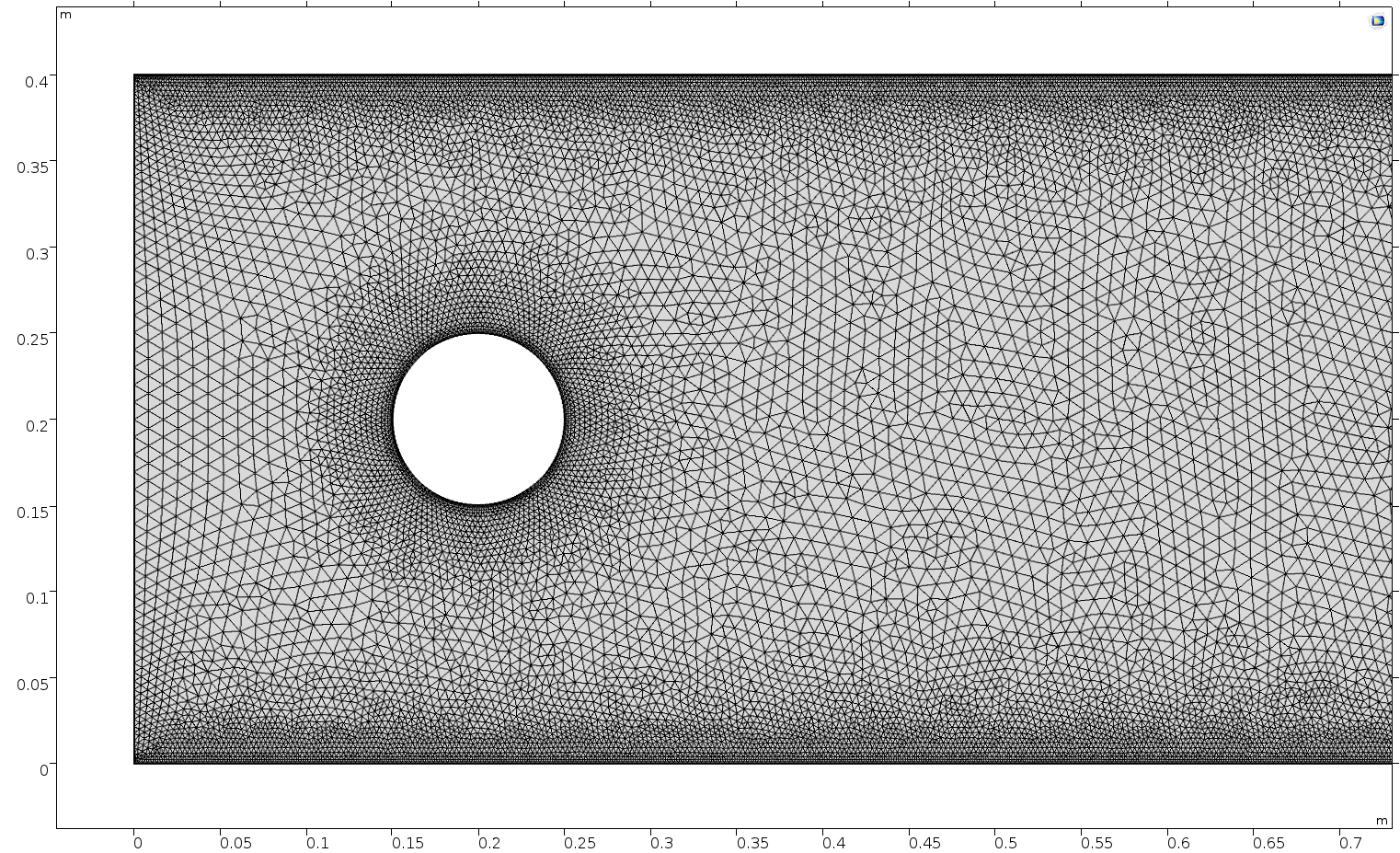
Below is the geometry of our simple model in COMSOL.
This is a two-dimensional COMSOL model, which assumes that the channel is of infinite depth and thus does not produce drag from the bottom of the flow in any way. Both the horizontal (long) walls and the walls of the cylinder have a "no slip" condition. This means that as the flow gets closer to the wall, velocity goes to zero. This condition sets up a velocity gradient between the walls at zero and the center of the flow. The wall on the far left side has an inflow condition of 1 meter per second, and the wall on the right side has a zero-pressure outlet condition, which lets flow pass out of the model unhindered.
COMSOL solves a finite element model, which means that it performs calculations for a mesh grid at each step. We use a relatively small mesh cell size ("Extra Fine" setting in COMSOL) on the order of ~1 cm.
When we run the model, we are executing a variation of the Navier-Stokes momentum equation for each mesh element of the model at each time step. This equation, shown above, is fundamental to describing the behavior of fluids in continuum mechanics.
Experimental variable: Viscosity
Let's look at the dynamic viscosities of fluids we'll be working with.
| Fluid | µ (viscosity at 20 ºC) |
|---|---|
| 1. Honey | 1 * 101.5 Pa s |
| 2. Water | 0.89 * 10-3 Pa s |
| 3. Air | 1.81 * 10-5 Pa s |
As mentioned above, we use an initial fluid velocity of 1 m/s in all of our models.
Questions to consider
From the diagram of the model geometry, what is the linear dimension (D)? In this model, it is equivalent to the diameter of the cylinder.
Before we go through the model results, try calculating the initial Reynolds numbers for each fluid viscosity using the linear dimension and the fluid velocity. Based on the Reynolds number calculated for the honey, do you think the fluid flow will be more laminar or turbulent? What about for water? Air?
Models
1) Honey (μ = 101.5 Pa s)
In the first example, we have a fluid with the viscosity of about that of honey, μ = 101.5 Pascal seconds (Pa s). You might imagine honey to be a pretty "stiff" liquid, which has something to do with its viscosity. What do you think will happen? Let's look at a few parameters of flow in the honey model.
Velocity 1 (x-component)
Things are pretty orderly and logical here. Not a whole lot changes over time. You might describe this flow system as "laminar," since you can describe what will happen at any given point in the model space at any given time fairly easily. Note that velocity is highest near the cylinder where the honey must "squeeze by" the cylinder in order to keep up with the 1 m s-1 inflow rate. This sets up a steep velocity gradient near the no-slip boundary of the cylinder, which we can see in the shear rate:
Shear rate 1
Shear rate is by definition the derivative of the velocity field, so it is no surprise that the highest shear values are in the areas next to the cylinder where the steep velocity gradient exists. If we break shear down into its component parts, we get vorticity. Vorticity is the curl of the velocity field, or in other words, the rate of rotation of the angle between two particles as they slip past each other.
Vorticity 1
Again, unsurprisingly, the curl is highest where the gradient of velocity is high. This makes sense because as two particles slip past each other at different velocities, their orientation changes (rotates) with regards to one another. Vorticity will be highest near the no-slip boundaries in a simple laminar system like this.
Pressure 1
The pressure field should also make sense, because our one obstacle in this model sets up the overall gradient from inflow to outflow pretty nicely. Notice that the pressure values are very slightly higher on the stoss side and slightly lower on the lee side of the cylinder. Note also that pressure gradients define the shortening and stretching of a system. Flow is shortened as it is forced towards the front of the cylinder and stretched as it goes past the cylinder.
Reynolds number 1
Reynolds number describes how chaotic a system is. Since our system has almost no chaos, this plot is pretty boring at this viscosity.
You may have noticed that the Reynolds numbers shown here are different orders of magnitude than those you calculated earlier. That's because the Reynolds numbers calculated via COMSOL are cell Reynolds numbers. This means that the Reynolds number is calculated using the characteristic length scale of the mesh grid size rather than the whole system. Despite this distinction, examining relative Reynolds numbers throughout the model will be useful for qualitatively describing what's happening with the flow.
Discussion 1 - Honey
Okay, so what's happening here? Things look pretty "boring" so far. With the exception of the very first couple of frames, in which the fluid has not achieved its full velocity yet, all of the frames are visually nearly the same. As you can tell by the color scale on the velocity plot, the fluid is moving as fast as 2 m s-1 past the cylinder, but there seems to be no instability here. This system is the result of kinematic forces at work, but the system seems to be stable, i.e. there is very little dynamic element to this system. Another way to say this is that there is not much variance in any given cell through time.
Why is this? Well, we said before that honey is "sticky." In more technical terminology, higher viscosity means higher internal friction and resistance to deformation. This has the effect of dampening the inertial term in Navier-Stokes, and thus causes the flow to gain stability and to behave in a "boring," predictable manner. Take another look at the Reynolds number plot. All areas on the plot are Cell Re < 1. The overall Re is on the order of 100.5 (around 3.2) since velocity is 1.0 m/s, the linear dimension or cylinder width is 10-1 m, and viscosity is 101.5 Pa s. This indicates a very stable and predictable flow, in which the kinematics of any one particle anywhere in the continuum can be described quite well mathematically. Let's take another look at the table we saw above:
| Quantifying qualitative descriptions of Reynolds number | ||
|---|---|---|
| Laminar | Transitional | Turbulent |
| Re < 100 | 100 < Re < 105 | 105 < Re |
Flows with Reynolds numbers of less than 100 are considered "laminar". This model shows laminar fluid flow around a cylinder.
2) Water (μ = 10-3 Pa s )
Now let's look at how flow changes when viscosity is lowered more than four orders of magnitude to that of water, μ = 10-3 Pa s (remember, we're holding density constant). What do you think will be different? What do you think the system will look like?
Velocity 2 (x-component)
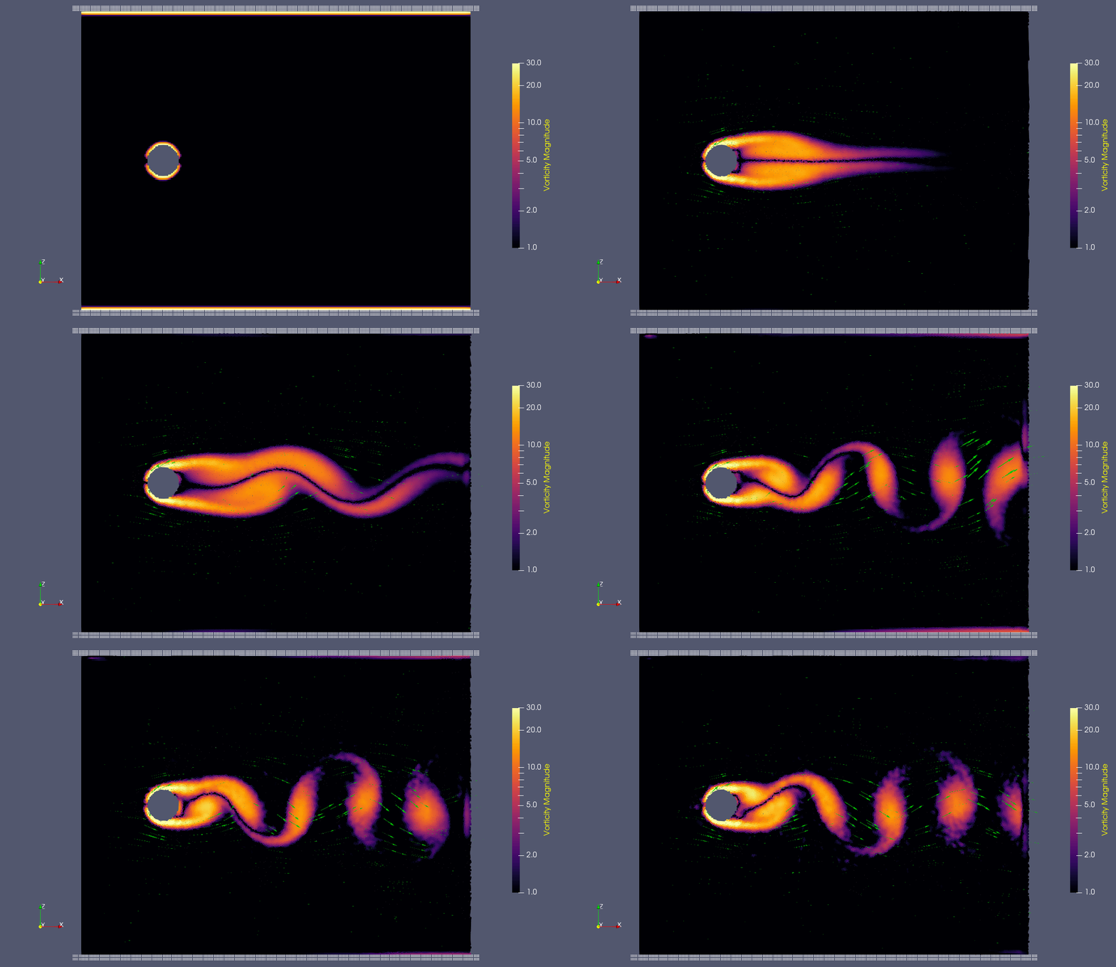
Whoa! That's quite different. Notice that things initially begin laminar but start to decay into a regular pattern of "wobbling." This process of vortex formation in the wake of the flow around the cylinder is called vortex shedding. Notice also how violently the velocity vectors swing around as the vortices begin forming and shedding and the flow field oscillates from side to side. Flow is actually going backwards in some places! Why?
There's no question this flow is more dynamic than the first one. Technically, as you'll see just below, this is still a laminar flow. Why? Can you still predict what's happening in certain places or at certain times? Why or why not? Keep these questions in mind as you scroll through the next few plots.
Shear rate 2
Here we see the shear plot, which still tracks the derivative of the velocity field, but in this case it's much more dynamic as well. We can see the formation of vortices as the dominant shear jumps back and forth between the two sides of the cylinder. Why do you think this is happening?
Vorticity magnitude 2
What a gorgeous vorticity plot. After you've admired it for a bit, can you describe what's happening here? Look back at the shear plot. When the newest vortex is about to detach from the lee side of the cylinder, where is the shear rate highest?
Pressure 2
Look at the similarities between this pressure plot and the vorticity plot, and you'll notice that pressure is more or less inversely related to vorticity. Why? Can you think of real-life scenarios (other than flow past a cylinder in a flume) where you can observe this phenomenon? Recall the flow vectors going backwards. Given this pressure plot, can you give an explanation for this phenomenon?
Reynolds number 2
Notice the change in magnitude of the cell Reynolds numbers calculated in this model. Recall that higher Reynolds numbers suggest more turbulent flow while lower Reynolds numbers indicate more laminar flow. Where do you see the most turbulent flow in the model? The least? Why do you think this is happening?
The overall Reynolds number for the system is 89. The Reynolds number doesn't quite make it above the critical number of 100 in order to be considered a "transitional" flow. What is happening in this flow that keeps it relatively "predictable?"
Note: The stippling is an artifact of the meshing process in COMSOL.
Discussion 2 - Water
The vortex shedding pattern shown in these examples develops after a couple of brief moments in which the flow is fairly laminar and there are few dynamics acting on the system. Then the system begins to develop an instability. In real life this instability is the result of tiny perturbations on the surface of the cylinder that cause differences in the boundary layer thickness as flow passes, causing one side to briefly slip faster than the other. The momentum of the vortex continues over to the other side of the cylinder, which increases the fluid pressure on that side and thus slows flow. As pressure always wants to equilibrate, this process reverses and a competing vortex is sent spinning to the opposite side. If flow conditions do not change, this process will continue indefinitely.
In mathematical terms, fluid particles will accelerate over time—∂v / ∂t—towards areas of low pressure—- ∇P (or decelerate if they are already traveling away from an area of low pressure). In order to figure out whether a particular particle will accelerate (or decelerate) towards a certain area of pressure, you'd have to examine the direction magnitude component partial differentials of the velocity and term, ∇2U. In other words, the grad (∇) symbol is a shorthand for the fact that you're looking at something that changes in more than one linear dimension (in the case of this simple 2D model, ∇ denotes that the variable will change in both x and y).
In a 3D model, the same patterns hold true. Let's look at a particle model of the same process. Particles in the first plot here are given colors based on the x component of their velocity.
In the second plot, particles are given colors based on their vorticity.
As a fluid becomes less viscous, the momentum term will begin to dominate the Navier-Stokes solution, meaning that the internal shear strength of the fluid is less able to keep it from deforming. As we said before, in this flow past a cylinder model, that means vortex shedding will become more and more viable at either lower viscosities or higher velocities.
Real-world applications
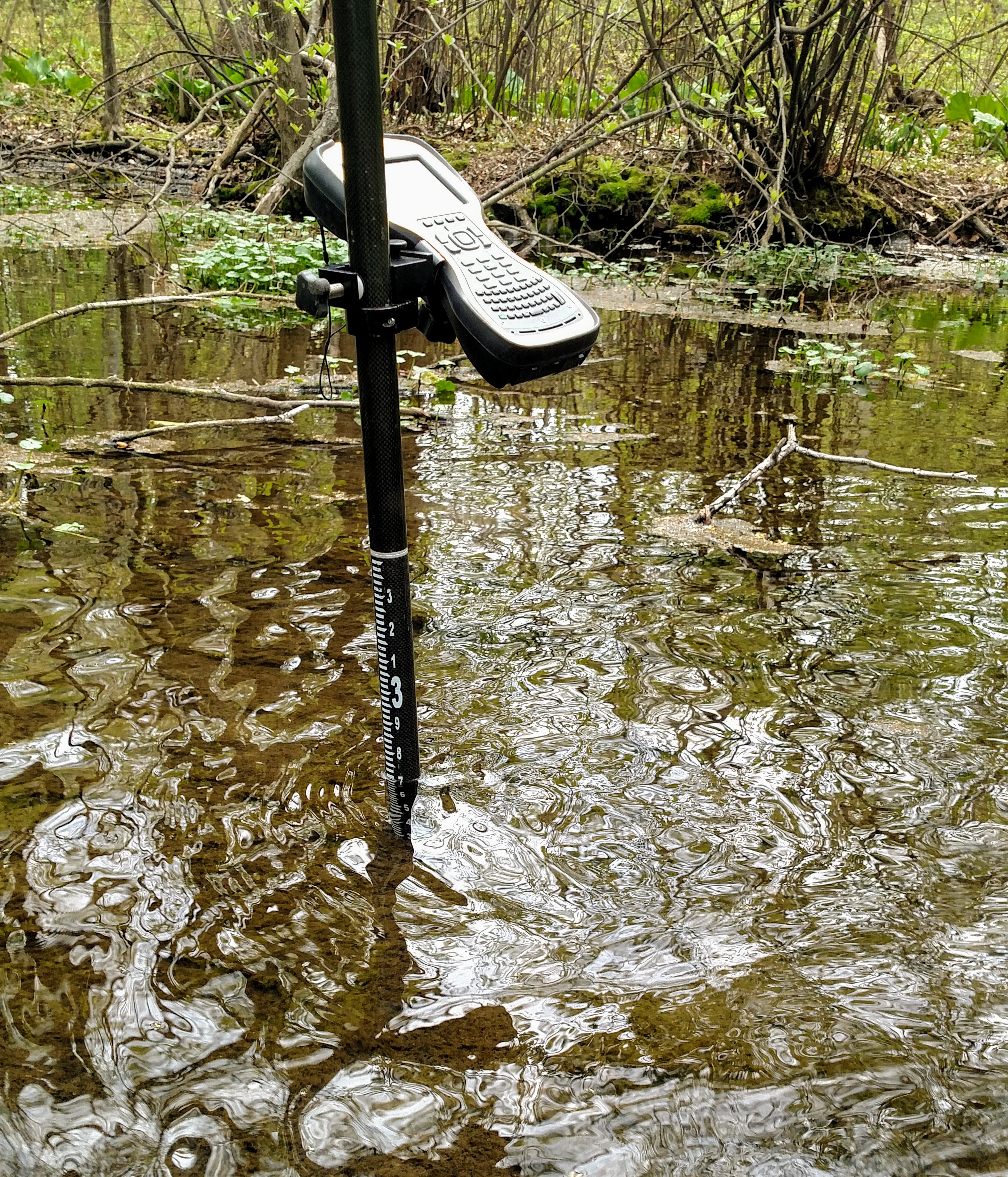
Pictured at right, a GPS survey staff causes a slight flow instability downstream.
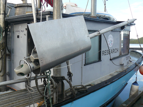
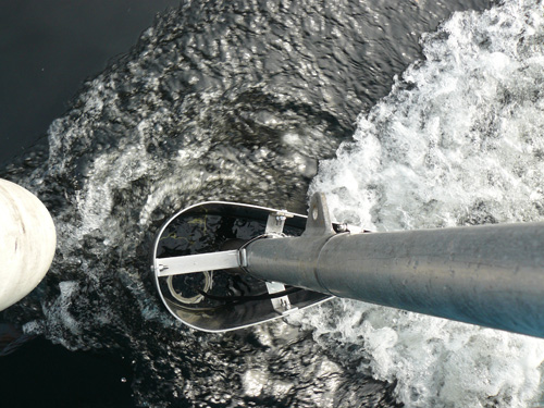
As beautiful as they are, von Kármán vortex streets are an engineering problem in many real-world applications. For example, the low pressure behind a cylindrical marine survey mount pole (pictured below) can cause more than 10 times more drag than a hydrodynamic shape like a teardrop. The vortex shedding can put enormous shear forces on the mechanical joints of a survey mount, which can cause brittle failure if they get high enough. Stainless steel "fairings" are sometimes used to reduce this drag and stop the pole from flexing.
Now, let's take a look at this behavior in a fluid with two orders of magnitude less viscosity than water: air.
3) Air (μ = 10-5 Pa s)
Air has a viscosity of μ = 10-5 Pa s (still holding density and velocity constant). How do you think this will affect the deformation of the fluid?
Velocity (x-component) 3
Shear rate 3
Vorticity magnitude 3
What is happening to the vorticity as the fluid moves further past the cylinder? Energy from the disturbance propagates forward and eventually dissipates. Can you see where this is happening from each of other variable plots as well?
Pressure 3
Reynolds number 3
Note: The stippling is an artifact of the meshing process in COMSOL.
Discussion 3 - Air
This specific type of oscillating flow is called a von Kármán vortex street (VKVS), named after Theodore von Kármán, the Hungarian-American physicist who first described it in detail. The process that leads to this type of flow is called vortex shedding. Let's take a deeper look at how these vortices are forming by looking at the particle solution generated in SPH.
These von Kármán vortex streets refer to the double row of vortices being shed from either side of the cylinder. The vortices formed from one side rotate in the opposite direction as the vortices formed from the other side. Each respective vortex row is referred to as a vortex street. Notice that angles at which the vortexes are moving relative to each other.
Compare the vortices here to those generated in the water flow around a cylinder model. What stands out to you about these vortices and what do you think is causing those differences? The ability of these vortices to maintain their form and stability through the entire simulation is remarkable. What do you notice about how they change over time and space? You may notice that these vortices are spaced differently and that they are different sizes than those from the water flow model. These VKVS can be described using several parameters:
The geometry of a VKVS can be defined by two dimensionless ratios, their aspect ratio and their dimensionless width. The aspect ratio is equal to h/a where h is equal to the separation distance between 2 the counter-rotating vortex streets and a is the the distance between 2 vortices in the same vortex street. What would you estimate this ratio to be for the vortices above? The dimensionless width of the VKVS is h/D where D is the diameter of the obstacle (cylinder in this case). In other words, the dimensionless width is just the ratio of the vortex street width to the width of the obstacle. What would you estimate the dimensionless width to be for the vortex street above? These parameters allow us to compare the geometry of vortex streets that vary vastly in size scale. The stable aspect ratio and dimensionless widths observed in lab settings are 0.28 and 1.2, respectively. How do these compare to those you calculated for this VKVS?
The vortex shedding frequency of a VKVS can be calculated from its Strouhal number, which describes the periodicity of oscillating flow mechanisms. The Strouhal number (St) is calculating using the frequency of vortex shedding (f), the obstacle/object diameter (D), and the flow velocity (u): St = f*D/u. Knowing the cylinder diameter (0.1 m) and the flow velocity (1.0 m/s), can you count the vortex shedding frequency from the animation to calculate the Strouhal number of this VKVS?
These von Kármán vortex streets are well-studied fluid phenomena that occur during the transition to turbulence (when 100 < Re < 105). Vortex shedding has many real-world engineering and design applications, some of which were described in the water flow discussion. Next, let's learn about their atmospheric counterparts!
Real-world Applications
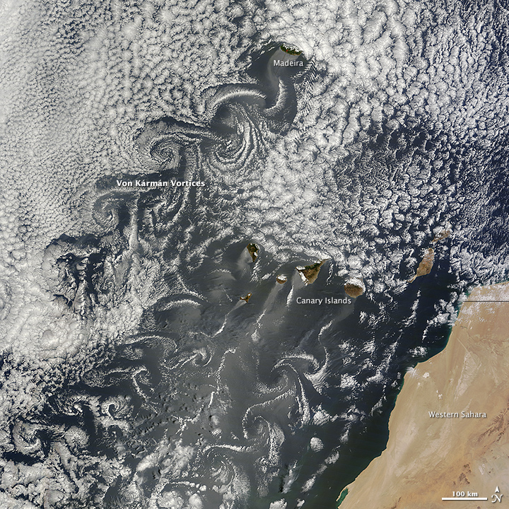
While von Kármán vortex streets have been thoroughly-modeled in lab settings, they occur naturally in the atmosphere. In fact, the first VKVS described by Theodore von Kármán were observed in the sky. He noticed remarkable swirling patterns in the clouds forming on the lee side of an island. These VKVS occur on a much larger scale than the VKVS that are modeled in lab settings. In the case of these atmospheric vortex streets, there are vertical forces, atmospheric pressure and temperature gradients, and a whole slough of other factors that influence the geometry and stability of the vortices. Many studies have modeled atmospheric VKVS such as the ones shown in the image to the right.
In the case of these atmospheric VKVS, the island acts as the cylinder in our fluid flow models, creating the flow disturbance. As air flows around the island obstacle, vortex shedding begins and these counter-rotating vortices propagate downwind. Do you notice any other differences between these atmospheric VKVS and the simulated VKVS from our air flow around a cylinder model?
Using the scale bar in the image above, measure the linear dimension (D) or width of Madeira. Using a wind speed of 10 m/s and the viscosity of air, can you calculate the general Reynolds number for flow around Madeira using the same steps as you previously did in the module?
Now use the same scale bar to measure and characterize the geometry of these atmospheric VKVS. What's the aspect ratio of the VKVS created by Madeira? The dimensionless width? How do these compare to those values observed in lab settings?
Conclusions
This module has introduced you to some of the tools that you can use to qualitatively and quantitatively characterize fluid flow as well as the physics behind it. The Navier-Stokes momentum equation governs the fluid particle motion while the Reynolds number describes the flow regime. The von Kármán vortex streets generated in the transition to turbulence can also be characterized by their aspect ratio, dimensionless width, and vortex shedding frequency (Strouhal number). Now that you have explored and described the transition to turbulence through models of fluid flow around a cylinder, you can use your knowledge to examine turbulence and flow behavior in other fluid systems!
Bonus: Complex flows
Although our module focused on models of simple fluid flow, more complex flows make up the vast majority of flow behavior you'll encounter in the real world. It's important to note that the systems modeled above above are highly simplified in order to highlight the physical forces acting on fluids. Below are some examples of more complex flow systems that one might encounter in the real world.
Fully turbulent flows
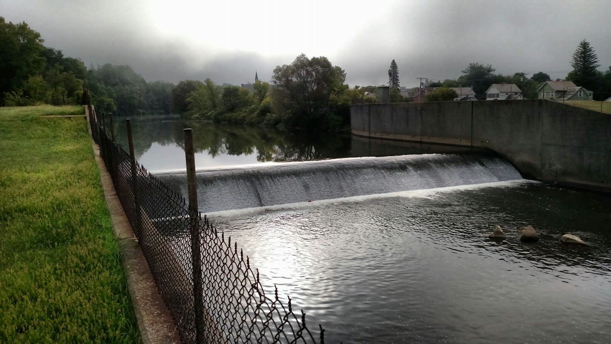
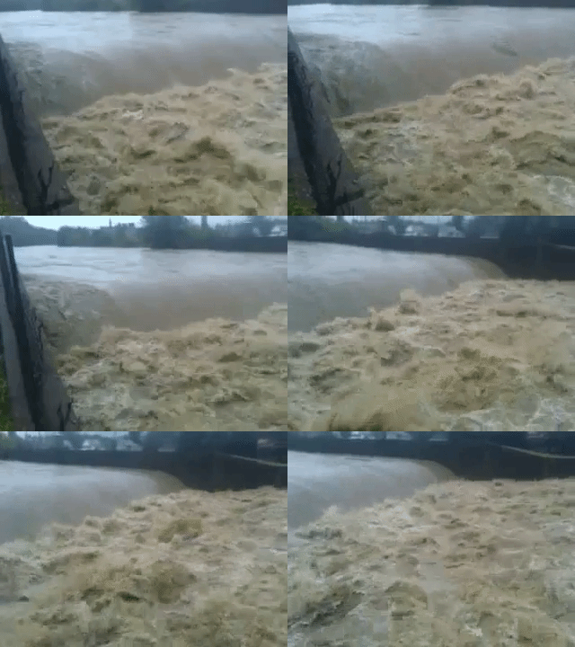
Fully turbulent flow, where 2000 < Re and predictability over a scale larger than a couple of particles or beyond a couple of time steps approaches zero, is very difficult to model. In some cases, flows of this nature are easier to compute and the solutions are better represented by Smoothed Particle Hydrodynamic models, in which individual particle smoothing kernels, rather than mesh elements, define the behavior of the fluid. However, flows in high Reynolds cases are are difficult to describe mathematically, and thus solutions that approach full turbulence in continuum or smoothed particle models can take orders of magnitude longer to compute.
The gif above was filmed on August 28, 2011, near peak flow during Hurricane Irene, the current flood of record for USGS gaging station 01332500 near Williamstown, MA. The video shows flow over a US Army Corps of Engineers (USACE) flood control structure (also pictured at baseflow on right). The concrete-bedded flood control flume has low bed roughness and thus high velocity, and comparatively lower Re. Flows like this can be very erosive when they encounter a jump in bed roughness due to a transition from a flood-control flume with a concrete bed to natural (rougher) bed conditions. The purpose of induced turbulence—from USACE's perspective—is to limit scour caused by a sudden increase in bed roughness. By increasing turbulence and thereby reducing friction at the boundary layer, the flow will not be quite as erosive in its transition between bed conditions. The flow captured in this video is at or near the flood control project's design capacity to limit the destructive nature of the flow, and thus this event still eroded cobble- and boulder-sized particles from the natural bed.
"Multiphase" flows
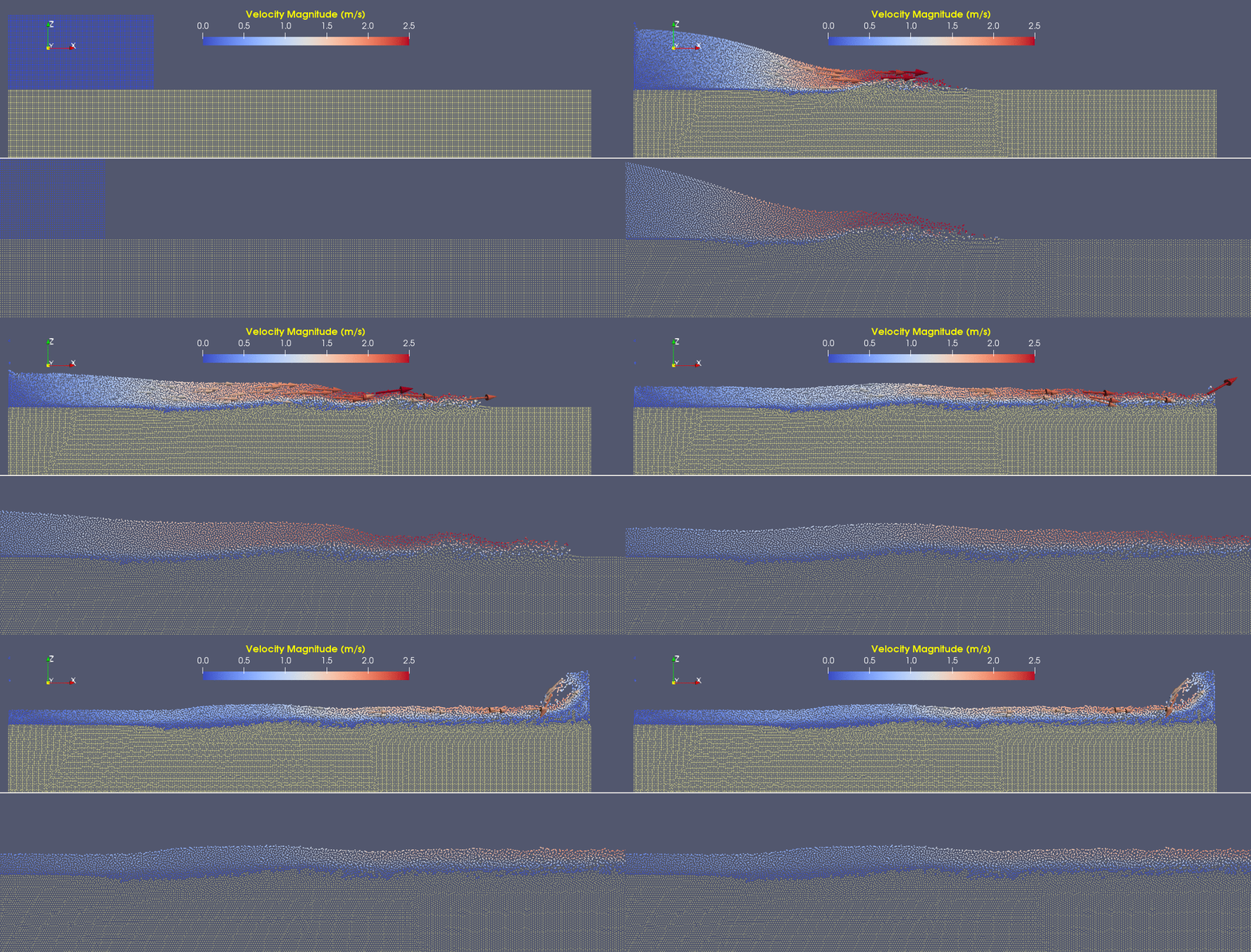
Using a particle physics solution, one can model fluid particle behavior without the need for computationally remeshing, which can have substantial processing power overhead in a continuum model. In this case we use the word "multiphase" to describe the use of two fluids, each with different properties, to initialize the model. The following GIF shows a DualSPHysics two-phase example model of a dam break, where a parcel of water flows over and deforms denser substrate (sediment) material. This type of model can be used to examine physical processes of erosion at a small scale, and potentially could be used to reproduce and expound on results of physical modeling studies of these phenomena.
As you can see here, water flowing on the surface of the sediment creates shear stress at the bed, which both deforms the sediment to certain depths, and entrains grains from the surface. You'll notice that as the front of the flow takes on sediment it behaves more like a debris flow than a water wave. This has the effect of buoying dense sediment up to the surface, which then remains entrained as the flow hits the wall and begins to curl around. From the DualSPHysics documentation:
These multi-phase sediment scouring phenomena are induced by rapid flows creating shear forces at the surface of the sediment which causes the surface to yield and produce a shear layer of sediment suspended particles at the interface and finally sediment suspension in the fluid. Applications include scouring in industrial tanks, port hydrodynamics, wave breaking in coastal applications and scour around structures in civil and environmental engineering flows among others.
Some of the more relevant physical properties of this model are shown in the following table.
| Fluid properties of multiphase model | |||||
|---|---|---|---|---|---|
| Fluid | Density (kg m-3) | Viscosity (Pa s) | Speed of sound (m s-1) | Cohesion coeff. | Angle of internal friction (deg) |
| Water | 1000 | 0.001 | 80 | 0 | 0 |
| Saturated sediment | 1500 | 0.002 | 81 | 1 | 35 |
A physical multiphase model typically involves a flume, a pump, and a specific particle size or range of sizes to test the effects that flow-induced boundary stress will have on particle saltation, sliding, and entrainment. A simple sediment flume demonstration conducted by Dr. Ronadh Cox (Williams College) is shown below. Apart from the geometry, one major difference between this physical model and the numerical one is that the grain density is that of quartz (2650 kg m-3) in the physical model.
