Topographic Anisotropy Figure 1
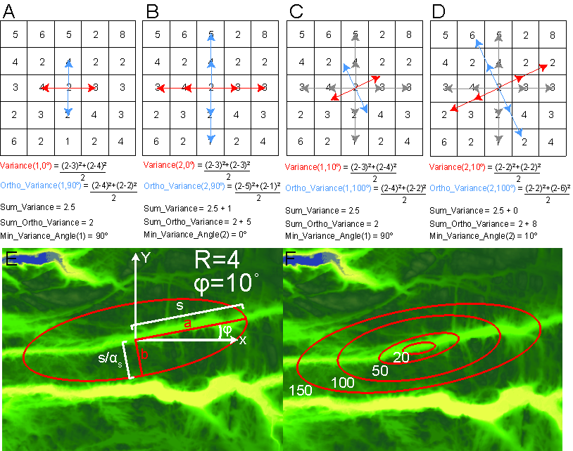
Figure 1: A) An example grid in which we apply our variance algorithm. Starting at with separation distance equal to the grid resolution, calculate variance between center point and points 0˚ and 180˚ and separation distance 1 away from center (red arrows). Also calculate variance for points orthogonal to 0˚ and 180˚ (blue arrows). B) Separation distance is doubled and variance values are calculated for the new scale. The variance for this scale is the average of the new variance and the variance calculated at the previous separation distance. C) Variance is now measured for and . The new variance value does not exceed the previously calculated value at the given scale and is therefore not used to measure anisotropy. D) The calculation is repeated at the second scale, variance is less than the previous calculation and so is now used to measure anisotropy for s = 2. E) Anisotropy is taken by dividing the minimum variance from the variance value measured at a perpendicular angle. The anisotropy value is the magnitude difference in variance for the two perpendicular directions, represented by an ellipse in the figure. F) The azimuth and magnitude of anisotropy is measured over multiple scales. Red ellipses represent topographic anisotropy magnitude (ellipticity), orientation (direction of semimajor axis), and wavelength (length of semimajor axis).
