Difference between revisions of "Transition to Turbulence"
(→Honey (μ = 101.5 Pa s)) |
(→Water (μ = 10-3 Pa s)) |
||
| Line 125: | Line 125: | ||
Flows with Reynolds numbers of less than 10 are considered "laminar," while those from 10 to 2000 are "transitional," and above 2000 "turbulent." | Flows with Reynolds numbers of less than 10 are considered "laminar," while those from 10 to 2000 are "transitional," and above 2000 "turbulent." | ||
| − | == Water | + | == Water == |
| − | Now let's look at how flow changes when viscosity is lowered more than four orders of magnitude to that of water (remember, we're holding density constant). What do you think will be different? What do you think the system will look like? | + | Now let's look at how flow changes when viscosity is lowered more than four orders of magnitude to that of water, μ = 10<sup>-3</sup> Pa s (remember, we're holding density constant). What do you think will be different? What do you think the system will look like? |
=== Velocity (x component) === | === Velocity (x component) === | ||
Revision as of 02:36, 22 February 2019
Created by Ian Nesbitt and Jukes Liu on 2019-02-19
Contents
Overview
In this module, you will learn how viscosity affects the dynamics of a simple fluid system with a single cylindrical impediment placed in the flow path. Our tools in this endeavor are COMSOL Multiphysics and ParaView. At the end of the module, you should be able to describe the initial conditions of a system, the transition from laminar to turbulent flow, and the effect viscosity has on the inertia, complexity, and predictability of a system.
We will move from looking at models with higher viscosity regimes and move to lower viscosity. Viscosity is the measure of a fluid's resistance to deformation.
First, let's start by learning how to talk about the various components of flow.
Basics
When we talk about flow, we need to first describe the fluid. Some of the fundamental characteristics of fluid are density, viscosity, compressibility, heat capacity, and thermal conductivity. In this exercise we will ignore the thermal properties entirely, define constant density and compressibility, and focus most of our attention on how viscosity affects the kinematics of a fluid system.
Compressibility and density are fairly easy to define. Compressibility is the tendency of a fluid to change its volume due to changes in pressure. Since we are not dealing with immense pressure, we assume that compressibility is zero across all models. Density is the quantity of mass per unit volume. For the purposes of this model, we will hold density constant at 1 kg m-3 to try and isolate the effects of viscosity.
These parameters will be fed into the Navier-Stokes fluid momentum equation (below) for each location in the model at each time step.
∂v / ∂t = ρg + µ∇2U - ∇P
| where | |
|---|---|
| ∂v | = change in velocity |
| ∂t | = change in time |
| ρ | = density |
| g | = acceleration due to gravity |
| µ | = viscosity |
| ∇2U | = divergence of velocity (gradient) |
| ∇P | = divergence of pressure (gradient) |
Since we are changing viscosity and looking at its effect on flow, let's look at the viscosities of fluids we'll be working with.
| Fluid | µ (viscosity at 20 ºC) |
|---|---|
| Honey | 1 * 101.5 Pa s |
| Water | 0.89 * 10-3 Pa s |
| Air | 1.81 * 10-5 Pa s |
Model
Below is the geometry of our simple COMSOL model.
This is a two-dimensional COMSOL model, which assumes that the channel is of infinite depth and thus does not produce drag from the bottom of the flow in any way. Both the horizontal (long) walls and the walls of the cylinder have a "no slip" condition. This means that as the flow gets closer to the wall, velocity goes to zero. This condition sets up a velocity gradient between the walls at zero and the center of the flow. The wall on the far left side has an inflow condition of 1 meter per second, and the wall on the right side has a zero-pressure outlet condition, which lets flow pass out of the model unhindered.
When we run the model, we are executing a variation of the Navier-Stokes momentum equation for each mesh element of the model at each time step. This equation, shown above, is fundamental to describing the behavior of fluids in continuum mechanics.
Honey
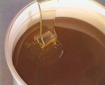
In the first example, we have a fluid with the viscosity of about that of honey, μ = 101.5 Pascal seconds (Pa s). You might imagine honey to be pretty "sticky," which has something to do with its viscosity. What do you think will happen? Let's look at a few parameters of flow in the honey model.
Velocity (x component)
Things are pretty orderly and logical here. Not a whole lot changes over time. You might describe this flow system as "laminar," since you can describe what will happen at any given point in the model space at any given time fairly easily. Note that velocity is highest near the cylinder where the honey must "squeeze by" the cylinder in order to keep up with the 1 m s-1 inflow rate. This sets up a steep velocity gradient near the no-slip boundary of the cylinder, which we can see in the shear rate:
Shear rate
Shear rate is by definition the derivative of the velocity field, so it is no surprise that the highest shear values are in the areas next to the cylinder where the steep velocity gradient exists. If we break shear down into its component parts, we get vorticity. Vorticity is the curl of the velocity field, or in other words, the rate of rotation of the angle between two particles as they slip past each other.
Vorticity
Again, unsurprisingly, the curl is highest where the gradient of velocity is high. This makes sense because as two particles slip past each other at different velocities, their orientation changes (rotates) with regards to one another. Vorticity will be highest near the no-slip boundaries in a simple laminar system like this.
Pressure
The pressure field should also make sense, because our one obstacle in this model sets up the overall gradient from inflow to outflow pretty nicely. Notice that the pressure values are very slightly higher on the stoss side and slightly lower on the lee side of the cylinder. Note also that pressure gradients define the shortening and stretching of a system. Flow is shortened as it is forced towards the front of the cylinder and stretched as it goes past the cylinder.
Reynolds number
Reynolds number describes how chaotic a system is. Since our system has almost no chaos, this plot is pretty boring at this viscosity.
Discussion

Okay, so what's happening here? Things look pretty "boring" so far. With the exception of the very first couple of frames, in which the fluid has not achieved its full velocity yet, all of the frames are visually nearly the same. As you can tell by the color scale on the velocity plot, the fluid is moving as fast as 2 m s-1 past the cylinder, but there seems to be no instability here. This system is the result of kinematic forces at work, but the system seems to be stable, i.e. there is very little dynamic element to this system. Another way to say this is that there is not much variance in any given cell through time.
Why is this? Well, we said before that honey is "sticky." In more technical terminology, higher viscosity means higher internal friction and resistance to deformation. This has the effect of dampening the inertial term in Navier-Stokes, and thus causes the flow to gain stability and to behave in a "boring," predictable manner. Take another look at the Reynolds number plot. All areas on the plot are Re < 1. This indicates a very stable and predictable flow, in which the kinematics of any one particle anywhere in the continuum can be described quite well mathematically. Reynolds number is a way of quantifying whether a flow is laminar, transitional, or fully turbulent. The table below lists the qualitative descriptions for each quantitative range.
| Quantifying qualitative descriptions of Reynolds number | ||
|---|---|---|
| Laminar | Transitional | Turbulent |
| Re < 10 | 10 < Re < 2000 | 2000 < Re |
Flows with Reynolds numbers of less than 10 are considered "laminar," while those from 10 to 2000 are "transitional," and above 2000 "turbulent."
Water
Now let's look at how flow changes when viscosity is lowered more than four orders of magnitude to that of water, μ = 10-3 Pa s (remember, we're holding density constant). What do you think will be different? What do you think the system will look like?
Velocity (x component)
Whoa! That's different. Notice how violently the velocity vectors swing around after the velocity begins oscillating from side to side. Flow is actually going backwards in some places! Why?
There's no question this flow is more dynamic than the first one. Technically, as you'll see just below, this is still a laminar flow. Why? Can you still predict what's happening in certain places or at certain times? Why or why not? Keep these questions in mind as you scroll through the next few plots.
Shear rate
Here we see the shear plot, which still tracks the derivative of the velocity field, but in this case it's much more dynamic as well. We can see the formation of vortices as the dominant shear jumps back and forth between the two sides of the cylinder. When the newest vortex is forming, where is the shear rate highest?
Vorticity magnitude
What a gorgeous vorticity plot. After you've admired it for a bit, can you describe what's happening here?
Pressure
Pressure is inversely related to vorticity. Why? Can you think of real-life scenarios (other than flow past a cylinder in a flume) where you can observe this phenomenon?
Reynolds number
As discussed above, the Reynolds number doesn't quite make it above the critical number of 10 in order to be considered a "transitional" flow. Why do you think this is? What is happening in this flow that keeps it relatively "predictable?"
The stippling is an artifact of the meshing process in COMSOL.
Air (μ = 10-5 Pa s)
Velocity (x component)
Shear rate
Vorticity magnitude
Pressure
Reynolds number
The stippling is an artifact of the meshing process in COMSOL.
Fully turbulent flow
Although our models don't show it here, we think it would be good to show some examples of fully turbulent flow, where 2000 < Re and predictability goes to zero. Because the flows in these models are difficult to describe mathematically, the solutions in continuum finite element models can take orders of magnitude longer to compute. In some cases, flows of this nature are easier to compute and better shown in Smoothed Particle Hydrodynamic models, in which individual particle smoothing kernels, rather than mesh elements, define the behavior of the fluid.
For this reason, one can model transitions to very violent flows without much extra overhead in terms of processing power.


